
Finding the Alpha - Predicting Currency Prices
I was interested in trying to identify any patterns in foreign exhange rates with the idea that there are inherent trends across prices due to market economics. In this article I explore Forex data, visualise some interesting correlations and end with building a successful model to predict the GBP to USD exchange rate.
Getting the Data
I decided the best datasets to use would be some historical spot rates between a large variety of currencies spanning economies of varying types and development stages. This was surpringly not as straightforward as I initially expected, with the type and scale of data not available to download very easily.
I decided I would collect the information myself, by webscraping a fairly reliable source of information. I found that this section of the Bank of England hosted the information I needed in well structured table.
After exploring a few pages on the site for different exchange rates, I discovered the URLs for the different pages followed a convenient pattern. This would make generating the URLs for all of the pages I need to scrape very easy to generate. I had recently started to use Scrapy as a crawling and scraping framework, and I was extremely pleased with the ease of setup and the native parallelisation it supports. With a list of pre-generated URLs to scrape, this would make the data collection process a breeze. I opened up a new project folder and initialised a new Scrapy project with
        $ mkdir currency_analysis && cd currency_analysis
        $ virtualenv venv
        $ source venv/bin/activate
        $ pip install scrapy
        $ scrapy init currency_analysis
I then write a function to generate all of the URLs I want to scrape.
        @staticmethod
        def build_start_urls():
            # start_urls = ['https://www.bankofengland.co.uk/boeapps/database/Rates.asp?TD=21&TM=Dec&TY=2018&into=GBP&rateview=D']
            start_date = date(2000, 1, 1)
            end_date = date(2018, 12, 21)
            delta = end_date - start_date

            currencies = ['GBP', 'USD', 'EUR']
            urls = set()

            for currency in currencies:
                for i in range(delta.days + 1):
                    this_date = end_date - timedelta(i)
                    weekno = this_date.weekday()

                    if weekno < 5: # if weekday
                        day = this_date.day
                        month = this_date.strftime("%b")
                        year = this_date.year

                        url = f'https://www.bankofengland.co.uk/boeapps/database/Rates.asp?TD={day}&TM={month}&TY={year}&into={currency}&rateview=D'
                        urls.add(url)

            scraped_urls = retrieve_scraped_urls()
            remaining_urls = urls - scraped_urls

            print(f'{len(scraped_urls)} scraped urls. {len(urls)} total urls. {len(remaining_urls)} remaining urls.')

            return list(remaining_urls)
I then scrape these pages, respecting all robots.txt, extract the information needed from the table and after making use of the Item Pipelines mechanism within Scrapy, yield the results into a local Postgres server.
        def parse(self, response):
            for el in response.xpath('//*[@id="editorial"]/table/tr'):
                day, month, year, base_currency = self.parse_url(response.url)
                target_currency = el.xpath('td/a/text()').extract_first()

                row_data = el.xpath('td/text()').extract()
                try:
                    target_spot_rate = row_data[0].strip()
                except:
                    target_spot_rate = None
                try:
                    target_52wk_high = row_data[1].strip()
                except:
                    target_52wk_high = None
                try:
                    target_52wk_low = row_data[2].strip()
                except:
                    target_52wk_low = None

                yield CurrencyScraperItem(
                        url=response.url,
                        day=day,
                        month=month,
                        year=year,
                        base_currency=base_currency,
                        target_currency=target_currency,
                        base_value=1,
                        target_spot_rate=target_spot_rate,
                        target_52wk_high=target_52wk_high,
                        target_52wk_low=target_52wk_low
                    )
EDA
I begin an exploration phase by pulling in the data into a Jupyter notebook using SqlAlchemy, and performing a few pieces of initial treatment. I notice dates are formatted as string and fix this with
        # date manipulation
        df['date'] = df.apply(lambda x: datetime.date(x['year'], x['month'], x['day']), axis=1)
        df['date'] = pd.to_datetime(df['date'])
        df['week'] = df['date'].dt.week
I rename certain values and replace with the ISO names of the currencies for cleaner visualiations with
        # rename values to ISO format
        currency_dict = {'Japanese Yen': 'JPY','Malaysian ringgit': 'MYR','New Zealand Dollar': 'NZD','Norwegian Krone': 'NOK','Polish Zloty': 'PLN','Russian Ruble': 'RUB','Saudi Riyal': 'SAR','Singapore Dollar': 'SGD','South African Rand': 'ZAR','South Korean Won': 'KRW','Swedish Krona': 'SEK','Swiss Franc': 'CHF','Taiwan Dollar': 'TWD','Thai Baht': 'THB','Turkish Lira': 'TRY','US Dollar': 'USD','Australian Dollar': 'AUD','Canadian Dollar': 'CAD','Chinese Yuan': 'Yuan','Cyprus Pound': 'CYP','Czech Koruna': 'CZK','Danish Krone': 'DKK','Estonian Kroon': 'EEK','Euro': 'EUR','Hong Kong Dollar': 'HKD','Hungarian Forint': 'HUF','Indian Rupee': 'INR','Israeli Shekel': 'ILS','Latvian Lats': 'LVL','Lithuanian Litas': 'LTL','Maltese Lira': 'MTL','Slovak Koruna': 'SKK','Slovenian Tolar': 'SIT','Sterling': 'GBP','Swedish Krona ': 'SEK','Brazilian Real': 'BRL','Austrian Schilling': 'ATS','Belgian Franc': 'BEF','Deutschemark': 'DEM','Finnish Markka': 'FIM','French Franc': 'FRF','Greek Drachma': 'GRD','Irish Punt': 'IEP','Italian Lire': 'ITL','Netherlands Guilder': 'NLG','Portuguese Escudo': 'PTE','Spanish Peseta': 'ESP'}
        df['target_currency'].replace('Latvian Lats\r\nCurrency joined the Euro on 01/01/2014', 'Latvian Lats', inplace=True)
        df['target_currency_symbol'] = df['target_currency'].apply(lambda x: currency_dict[x])
        df.drop(columns=['target_currency'], inplace=True)
and finally drop unnecessary columns and reorder remaining columns, and I am left with clean dataframe to start some analysis.
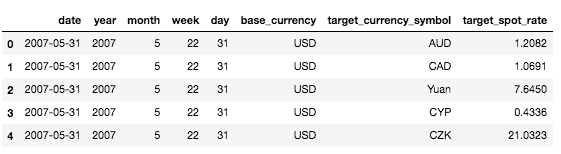
Dataframe snapshot
You can read the dataframe by taking the first row and saying that on 31st of May 2007, you could purchase 1.2082 Australian Dollars with 1 US Dollar at market close.
As a sanity check, I plot historical exchange rate data and cross check the data displayed in the Notebook with XE.com, a service provider that shows exchange rates. Reassuringly, I find the data that I have collected matches data found elsewhere.
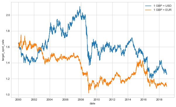
Historical GBP forex price
My next step was to try to find out if I could identify some trends in the data that I would be able to utilise in building a predictive model. With the information I have collected, I derive two additional types of data that explains different market phenomena’s; the relative price changes of a currency, sometimes called a return, and the volatility of price changes of a currency. To calculate returns, I needed to calculate the percentage difference of spot rates of a given currency, looking over a daily, weekly, monthly, and a yearly period. Due to the lack of price data on certain non-trading days such as weekends and bank holidays, I resampled the data to carry over the price of a currency from the previous existing date - this approach is one of several that can be taken. I implemented this using Pandas resampling method over the different length periods I wanted returns over, demonstrated like this
        # add in data for missing dates
        currency_df = currency_df.sort_values(['date'])
        currency_df.set_index('date',inplace=True)
        currency_df = currency_df.resample('D', axis=0).pad()
        currency_df = currency_df.reset_index()
From here on, I look at data that has GBP as its base currency, that is all spot rates will refer to the amount of foreign currency I can purchase with £1.
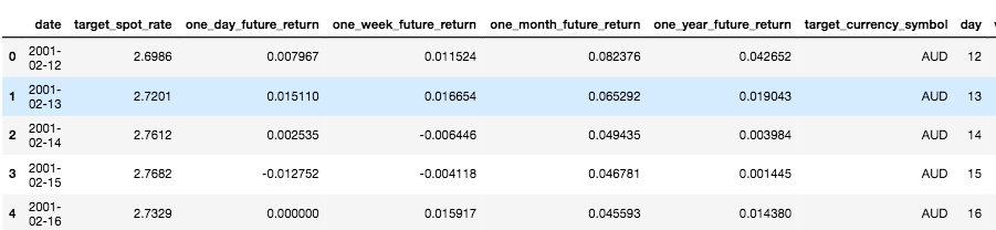
Analysis dataframe
What's important to notice here is that the resulting DataFrame will give us, say the spot rate on any given day, as well as the percentage increase of price based on a future price. I.e. If on the 12th February 2001 I can buy 2.6986 Australian Dollars with 1 GBP, the monthly return column shows us that in one months' time, on 12th March 2001, the price will be 0.82% higher. This feature will allow us to use current data such spot rates and volatility to determine future price. Using a similar method, I calculate returns up to any given date as well, so we can use historical returns to predict future returns.
To derive price volatility, I took a simpler approach. All I needed to was group by price and the period over which I wanted to analyse and calculated the standard deviation in the target spot rates. In future analysis, this will change to grouping by the previous n-days rather than my current method.
        week_vol = currency_df.groupby(['week', 'month', 'year', 'target_currency_symbol'])['target_spot_rate'].std()
        week_vol = week_vol.reset_index().rename({'target_spot_rate': '1w_vol'}, axis=1)

        month_vol = currency_df.groupby(['month', 'year', 'target_currency_symbol'])['target_spot_rate'].std()
        month_vol = month_vol.reset_index().rename({'target_spot_rate': '1m_vol'}, axis=1)

        year_vol = currency_df.groupby(['year', 'target_currency_symbol'])['target_spot_rate'].std()
        year_vol = year_vol.reset_index().rename({'target_spot_rate': '1y_vol'}, axis=1)

        currency_df = currency_df.merge(week_vol, how='left', on=['week', 'month', 'year', 'target_currency_symbol'])
        currency_df = currency_df.merge(month_vol, how='left', on=['month', 'year', 'target_currency_symbol'])
        currency_df = currency_df.merge(year_vol, how='left', on=['year', 'target_currency_symbol'])
I then reshape the data so that each row represents a particular date and I can use prices and price volatilities of all currencies to predict returns in all currencies. The resulting dataframe looks like this
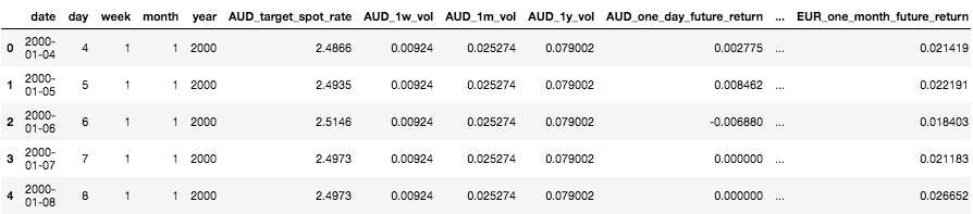
Reshaped dataframe
To quickly identify any interesting trends, I plot a correlation matrix of data, to determine if there are any linear relationships between returns and prices/volatilities.
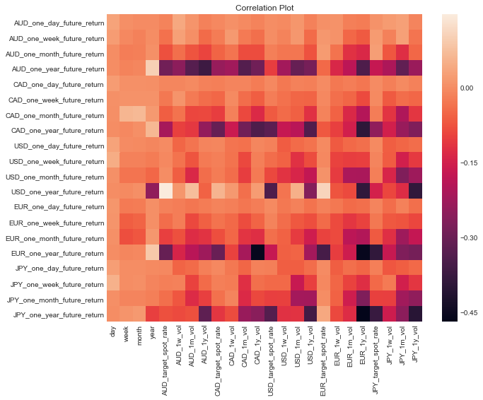
Correlation plot forex returns
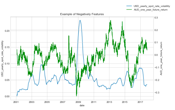
Any particular dark or light patches in this plot would indicate a trend between the two variables. For example, the one year return on GBP to Japanese Yen is correlated with the annual volatility between the GBP and the Euro. This is confirmed by plotting these two negatively correlated variables.
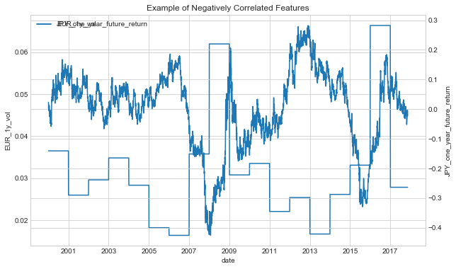
Negatively correlated features
It's clear that the lack of a more sophisticated approach to calculating volatility may be affecting the results, so
I try to address this now.
I fix this problem by taking advantage of the rolling method of a DataFrame with a DateTimeIndex
that allows calculations over certain periods of time.
This is a simple and effective fix and much simpler implementation than the one used to calculate returns. Here is
the updated correlation matrix along with some interesting correlations.
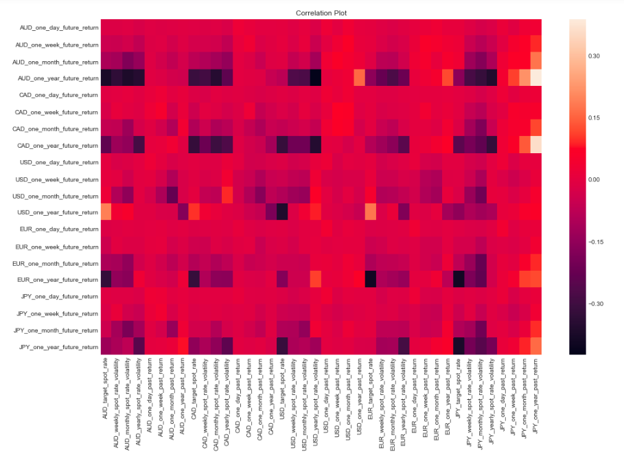
Updated correlation plot
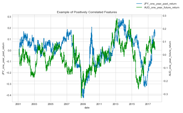
Positively correlated features
Negatively correlated features
To find the distribution of each variable, I use a handy function I have written that shows the distribution of all columns of a DataFrame to be shown in a single plot.
        import math
        def plot_matrix_of_graphs(graph_func, df, cols, n=6, title=''):
            """
            :param graph_func: plotting function
            :param df: dataframe
            :param cols: columns to plot
            :param n: number of rows in plot viz matrix
            """
            temp_df = df.dropna()
            m = math.ceil(len(cols)/n)
            fig, axes = plt.subplots(n, m, figsize=(20, 15))
            plt.subplots_adjust(hspace=0.5)

            i, j = 0, 0

            for col in cols:
                graph_func(temp_df[col], ax=axes[i, j])
                j += 1
                if j >= m:
                    j = 0
                    i += 1

            fig.suptitle(title)
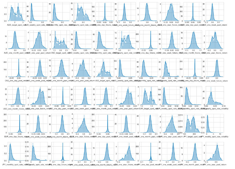
Histogram plots
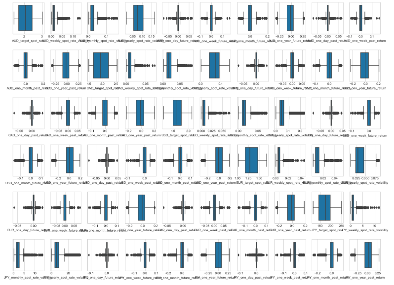
Box plots
These are two plots that I generate using the above function and the distplot and boxsplot
methods of Seaborn.
We can see here there are heavy skews in some variables and significant outliers in others. When modelling, I will
try to fit the model to the raw data and if there is no convergence, I will remove significant outliers and then
normalise the data.
Building Predictions
I decided that the label I wanted to start of by attempting to predict the annual return on the GBP to USD exchange rate so I remove the target variable from the DataFrame. I also drop all columns that refer to all other future returns since I will not have this data at hand when making predictions in real life. I split the data into train and test sets and loop through a few models I expect to give positive results, utilising cross validation sets.
        from sklearn.model_selection import train_test_split
        from sklearn.model_selection import cross_val_score
        from xgboost import XGBRegressor
        from sklearn.linear_model import LinearRegression, Ridge, Lasso

        models = [
            XGBRegressor(),
            LinearRegression(),
            Ridge(),
        ]

        X_train, X_test, y_train, y_test = train_test_split(X, y, test_size=0.20, random_state=42)

        k_folds = 3
        model_scores = []
        for model in models:
            model_name = model.__class__.__name__
            accuracies = cross_val_score(model, X_train, y_train, scoring='r2', cv=k_folds)
            for accuracy in accuracies:
                model_scores.append([model_name, accuracy])

        df = pd.DataFrame(model_scores)
        ax = sns.boxplot(x=0, y=1, data=df)
        ax.set_title('R-Squared on Models Predicting Annual Return on GBP:USD Rate')
This results in the following plot, which shows the XGBoost is the most suitable algorithm for this particular problem. I then confirm this by evaluating the accuracy on the test set, achieving a 0.96 score. The relatively high score may indicate a case of overfitting; however I do not address this problem now. To get a quick idea of feature importance, I use a library called SHAP. I will explain the various uses of SHAP and other methods of interpreting models in another blog post.
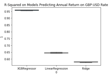
Regression model results on annual data
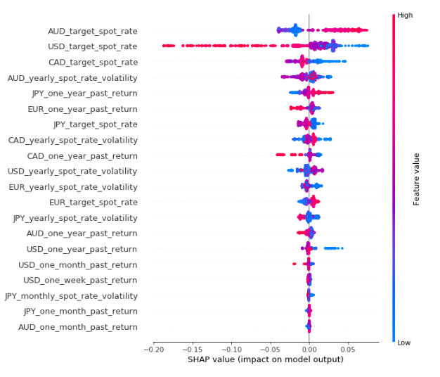
Feature importance
I then change the target variable to the monthly return on the GBP:USD rate since this would be considerably more
difficult to predict. Unsurprisingly, the model is less accurate, however still has significant predictive power at
being able to explain 0.65 of the observed variance. With a bit of hyperparameter tuning, I find that the model
XGBRegressor(max_deph=5, learning_rate=0.2, n_estimators=150) achieves 0.83 score.
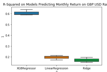
Regression model results on monthly data
I then translate this into a classification problem by relabelling the target variable as being True if we see positive returns and False if see non-positive returns. Important to note that when looking at monthly return, the classes are fairly well balanced. Here is the result along with a confusion matrix and a model summary.
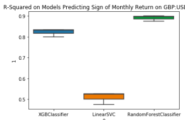
Classification model results on monthly data
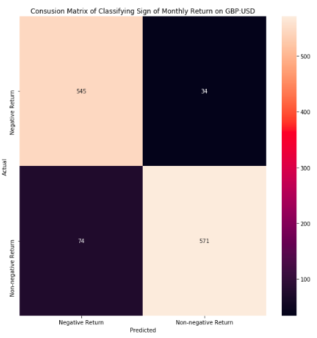
Confusion matrix
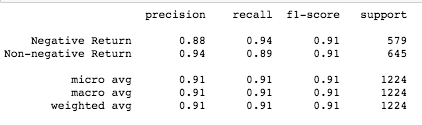
Classification report
In this case, the RandomForestClassfier method works the best of these three algorithms and produced an
accuracy score of 0.91 on the test set, and sees positive results for both of the predictor classes.
Conclusion
Analysis has shown that there is significant predictive power in the collected and derived data in being able to predict annual and monthly GBP:USD rates, with the former being more successful. There is also interesting, however mostly likely non causual relationships between some exchange rates and price volatility. All the code can be found on Github and you are encouraged to play around and see if you can find similar results for other currencies.